zrw2o8 pdf adps
ZrW2O8 PDF fitting with anisotropic displacement parameters
Files needed: zrw2o8_topas_sim_gr.xy, zrw2o8_pdfgui_sim_gr.xy, zrw2o8_start.cif, zrw2o8_ideal_adps_300k.cif
Learning outcomes: this tutorial describes three ways of modelling atomic displacement parameters for small box PDF fitting in TOPAS – one isotropic and two anisotropic. In the first anisotropic method a conventional Uij description is used, similar to that implemented in programs such as PDFGui. In the second the ADP_5 atomlet approach is used. The ideas behind this will be described in a paper by Alan and John.
The tutorial uses two data sets. The first is simulated with ideal Uij values for ZrW2O8 in TOPAS from reciprocal space data. It inherently includes low-r peak asymmetry due to anisotropic motion. The second is simulated in PDFGui and doesn’t take peak asymmetry into account.
Isotropic model
1. In topas-editor select a PDF fitting template from the “TOPAS_Durham/PDF Fitting” menu. Go through and update the lines starting with purple arrows (->). Set the filename to zrw2o8_topas_sim_gr.xy. Use the “Structure from CIF for PDF” to read in zrw2o8_start.cif. Set the cubic cell parameters to refine with equated values. Fit the data from 0.5 to 50 A. Note that the weighting function used puts zero weight on values below 1.5 A such that the PDF is calculated here but doesn’t influence the refinement. Set to refine an isotropic bvalue on each site.
2. Refine the atomic coordinates according to symmetry. To save typing you could copy the lines below. You should get an Rwp ~9.4%.
		site Zr1 x xZr1 0.00 y xZr1 0.00 z xZr1 0.00 occ Zr 1 beq @ 1
		site W1  x xW1  0.34 y xW1  0.34 z xW1  0.34 occ W  1 beq @ 1
		site W2  x xW2  0.60 y xW2  0.60 z xW2  0.60 occ W  1 beq @ 1
		site O1  x xO1  0.21 y yO1  0.44 z zO1  0.45 occ O  1 beq @ 1
		site O2  x xO2  0.79 y yO2  0.57 z zO2  0.56 occ O  1 beq @ 1
		site O3  x xO3  0.49 y xO3  0.49 z xO3  0.49 occ O  1 beq @ 1
		site O4  x xO4  0.23 y xO4  0.23 z xO4  0.23 occ O  1 beq @ 1
3. Save a copy of the refined sites in a /* comment */ in case you need to return to them.
Anisotropic displacement parameters – Uij
4. Try using anisotropic displacement parameters by replacing the “beq…” text at the end of each site line by “adps. To be safe you might want to fix atomic coordinates. Or you could use the same trick as in earlier tutorials and set the sites to refine with min/max values restricted to lie close to reference values. To do this highlight the sites (before changing to adps) and do: right-click/topas-editor commands/topas refine atomic coordinates. It will create a section something like the one below.
prm !max_shift 0.5 'Angstroms along each axis
macro Nvrx(name, value, ref) {x name value min = ref-max_shift/Get(a); max = ref+max_shift/Get(a);}
macro Nvry(name, value, ref) {y name value min = ref-max_shift/Get(b); max = ref+max_shift/Get(b);}
macro Nvrz(name, value, ref) {z name value min = ref-max_shift/Get(c); max = ref+max_shift/Get(c);}
macro Uii_ { min 0.00001 max 0.3 val_on_continue = Limit(Val + Rand(-1, 1) .001, 0.0001, .3); }
macro Uij_ { min -0.3 max 0.3 val_on_continue = Limit(Val + Rand(-1, 1) 0.001, -.1, .1) ; }
site Zr1  Nvrx(xzr1, 0.00123`,0.00122) Nvry(xzr1, 0.00123`,0.00122) Nvrz(xzr1, 0.00123`,0.00122) occ Zr   1   adps
site W1   Nvrx(xw1,  0.34108`,0.34111) Nvry(xw1,  0.34108`,0.34111) Nvrz(xw1,  0.34108`,0.34111) occ W    1   adps
site W2   Nvrx(xw2,  0.60029`,0.60033) Nvry(xw2,  0.60029`,0.60033) Nvrz(xw2,  0.60029`,0.60033) occ W    1   adps
site O1   Nvrx(xo1,  0.20651`,0.20651) Nvry(yo1,  0.43798`,0.43798) Nvrz(zo1,  0.44712`,0.44712) occ O    1   adps
site O2   Nvrx(xo2,  0.78717`,0.78717) Nvry(yo2,  0.56882`,0.56882) Nvrz(zo2,  0.55647`,0.55647) occ O    1   adps
site O3   Nvrx(xo3,  0.49156`,0.49155) Nvry(xo3,  0.49156`,0.49155) Nvrz(xo3,  0.49156`,0.49155) occ O    1   adps
site O4   Nvrx(xo4,  0.23307`,0.23306) Nvry(xo4,  0.23307`,0.23306) Nvrz(xo4,  0.23307`,0.23306) occ O    1   adps
5. The model should converge to Rwp ~2.7%. If you add the following two lines you can view the adps in vesta. They should be very similar to the reference values in the CIF used for simulation.
         Out_CIF_STR(zrw2o8_uij.cif)
         Out_CIF_ADPs(zrw2o8_uij.cif)
6. Keep a copy of the Uij coordinates in a /* comment block */.
7. You might also try fitting zrw2o8_pdfgui_gr.xy with this same model. You should get Rwp ~0.75% and a “perfect” fit and adps the same as in zrw2o8_ideal_300k.cif. This confirms that the TOPAS Uij routines give the same answer as those in PDFGui.
Anisotropic displacement parameters ADP_5
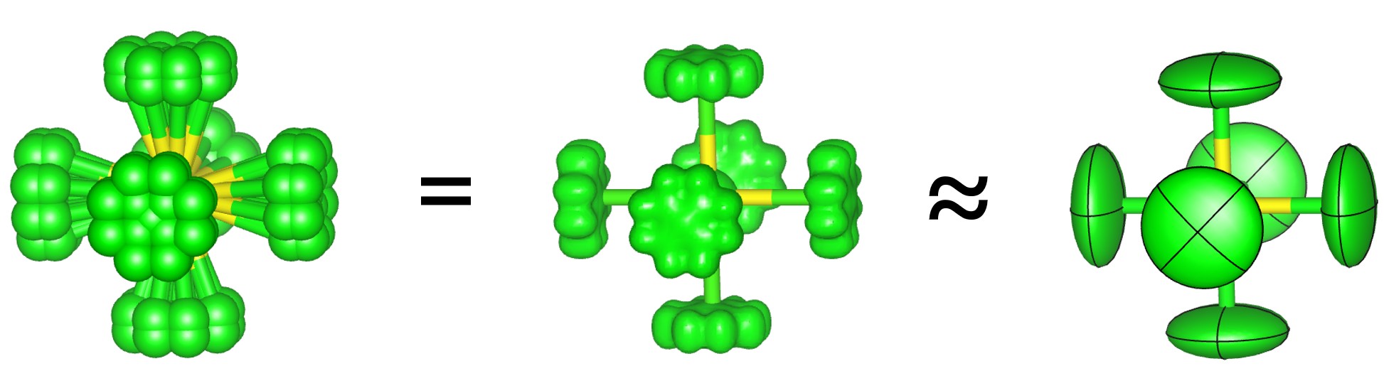
We will now use an ADP_5 model. This replaces single atoms with five atomlets which describe the distribution of atoms. The multiple interactions can inherently describe peak asymmetry.
8. The easiest way to create an ADP_5 model is to use a built in macro to describe each site’s atomlets. In topas-editor you can create this automatically. Copy the list of isotropic atoms given above or those in your INP file. In topas-editor highlight just these site lines and type shift-ctrl-p. This brings up the vs code command prompt. Start typing “adp_5” and select the command for converting format that is suggested. You should get a section in your INP file that looks like the one below. Note that you have to set the parameter names for fractional coordinates of the first site listed so they obey symmetry. e.g. for Zr1 make the first three values all xZr1. The x1,y1,z1 and x2,y2,z2 coordinates that describe other atomlets are handled automatically.
'macros to restrict and randomize ADP_5 coordinates
'*Warning: you will need to fix coordinate parameter names to obey site symmetry
'*Warning: any Get(x) equations will be interpreted incorrectly
#include ROOT##PDF-adps.inc 'uncomment this line if PDF-adps.inc not already included
macro R_ { min -0.05 max 0.05 val_on_continue = Rand(-1, 1) 0.01; }
ADP_5( Zr1, xZr1, 0.00108161192`, xZr1, 0.00108161192`, xZr1, 0.00108161192`, Zr, !occZr, 1, x1Zr1,-0.00633500818` R_, y1Zr1,-0.00611339955` R_, z1Zr1,-0.018403283` R_, x2Zr1,-0.00851042179` R_, y2Zr1, 0.00607363764` R_, z2Zr1,-0.00367342885` R_, boZr1, 0.414287686`)
ADP_5( W1, xW1, 0.34073204`, xW1, 0.34073204`, xW1, 0.34073204`, W, !occW, 1, x1W1, 0.000696930403` R_, y1W1,-0.00211578168` R_, z1W1, 0.000699002998` R_, x2W1, 0.00356758644` R_, y2W1, 0.0210020085` R_, z2W1, 0.00907151013` R_, boW1, 1.05476371`)
ADP_5( W2, xW2, 0.600319438`, xW2, 0.600319438`, xW2, 0.600319438`, W, !occW, 1, x1W2,-0.00567266553` R_, y1W2, 0.00760614805` R_, z1W2,-0.00405026456` R_, x2W2,-0.00687790244` R_, y2W2, 0.00541699054` R_, z2W2, 0.00374378009` R_, boW2, 0.630909549`)
ADP_5( O1, xO1, 0.206204262`, yO1, 0.438098424`, zO1, 0.446984044`, O, !occO, 1, x1O1, 0.00358713724` R_, y1O1, 0.0206471664` R_, z1O1,-0.0081095876` R_, x2O1,-0.00854814052` R_, y2O1,-0.00741267287` R_, z2O1,-0.018733841` R_, boO1, 0.864485374`)
ADP_5( O2, xO2, 0.787192304`, yO2, 0.568812027`, zO2, 0.556444459`, O, !occO, 1, x1O2,-0.00394233001` R_, y1O2, 0.00663539284` R_, z1O2,-0.013655637` R_, x2O2, 0.00938372687` R_, y2O2, 0.0215469252` R_, z2O2, 0.00778713409` R_, boO2, 0.723348829`)
ADP_5( O3, xO3, 0.491863016`, xO3, 0.491863016`, xO3, 0.491863016`, O, !occO, 1, x1O3,-0.0247434539` R_, y1O3, 0.00510775613` R_, z1O3, 0.0204186467` R_, x2O3,-0.00645767524` R_, y2O3,-0.00627188465` R_, z2O3, 0.0148141958` R_, boO3, 0.833895354`)
ADP_5( O4, xO4, 0.233149851`, xO4, 0.233149851`, xO4, 0.233149851`, O, !occO, 1, x1O4, 0.0193794194` R_, y1O4,-0.0300699342` R_, z1O4, 0.014682497` R_, x2O4, 0.0076775076` R_, y2O4, 0.00820394179` R_, z2O4,-0.0130815387` R_, boO4, 1.37135103`)
9. Refine with this model. You should get Rwp ~1.5%, an excellent fit to the data. The ADP_5 gives a better fit than the Uij model as it can describe low-r asymmetry.
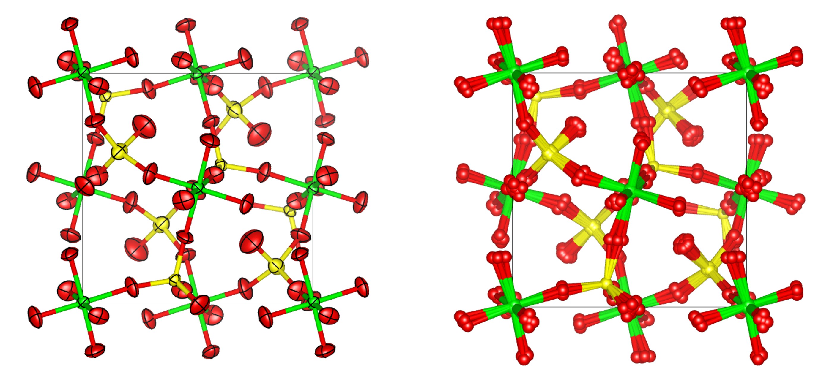
10. Add the command “view_structure” to the str section. You should see a model that looks something like the image below. The image compares 90% probability surfaces for the anisotropic displacement parameters in the ideal structure with the atomlet positions from the ADP_5 model. The figure shown is actually from a fit to experimental data.
11. Read the paper for more detail on the pros and cons of the ADP_5 model.
There is a cheat file here which is set up so you can try the three different models by commenting in/out sections with “#define use_uiso” etc.
Peak Broadening PDFGui and TOPAS
PDFGui broadens peaks using parameters delt1, delt2 and Qbroad. According to the manual uij‘=uij * Sqrt(1 – delt1/rij – delt2/rij2 + Qbroad2rij2). The lines below give exactly the same broadening in TOPAS for either uij sites or beq sites.
Note also that a Qdamp of 0.001 in PDFGui is equivalent to dQ_damping(!dQ, 0.00235482) in TOPAS (scale by * 2.35482).
uij sites need “adps_scale” equation after each site:
prm !delt1  0.75 vc min 1e-9 max 5
prm !delt2  0.25 vc min 1e-9 max 1
prm !Qb  0.05 min 1e-9 max 100
adps_scale = 2 aa (Abs(1 - delt1 / X - delt2 / X^2 + (Qb^2) X^2));
beq sites can use the following (note this is different to PDF.inc):
site O1 x   0.00000_ y   0.00000 z   0.00000 occ O 1 Beqpdfgui2(bval, 0.2368)
macro Beqpdfgui2(c, v)
   {
      #m_argu c
      If_Prm_Eqn_Rpt(c, v, min 1e-6 max 5 val_on_continue = Val Rand(.1, 2); )
      beq = CeV(c, v)   (Abs(1 - delt1 /(1e-10+X) - delt2 /(1e-10+X)^2 + Qb^2 X^2));
   }