tutorial vscode_riet_pawley

Rietveld and Pawley refinements using topas-editor

Learning Outcomes: This example goes through the mechanics of Rietveld and Pawley refinements in topas-editor/VS Code using TiO₂ lab data. Later tutorials cover more of the “why” behind each stage.

It’s written as a “first use of TOPAS”, so contains more screenshots than other tutorials. It assumes you have VS Code and the topas-editor extension installed and have a valid TOPAS license (TA or Bruker).

Rietveld refinement from scratch

1. Save the raw datafile and cif file in your working directory. Use “right click/save link as”. Don’t save the files in your main TOPAS directory.

2. Launch VS Code. If topas-editor is set up correctly your screen will look like the image below. Click on the image (and later images) to zoom. If you’re new to topas-editor click on “Topas-editor help” in the “COMMANDS VIEW” grey side menus for some tips. There is general help on TOPAS and links to various resources via the “Help/General Links” menu. If you don’t see the grey menus on the left, click on the white “triangle in circle” icon in the black side activity bar. It is highlighted by a white line to the left in the image below.

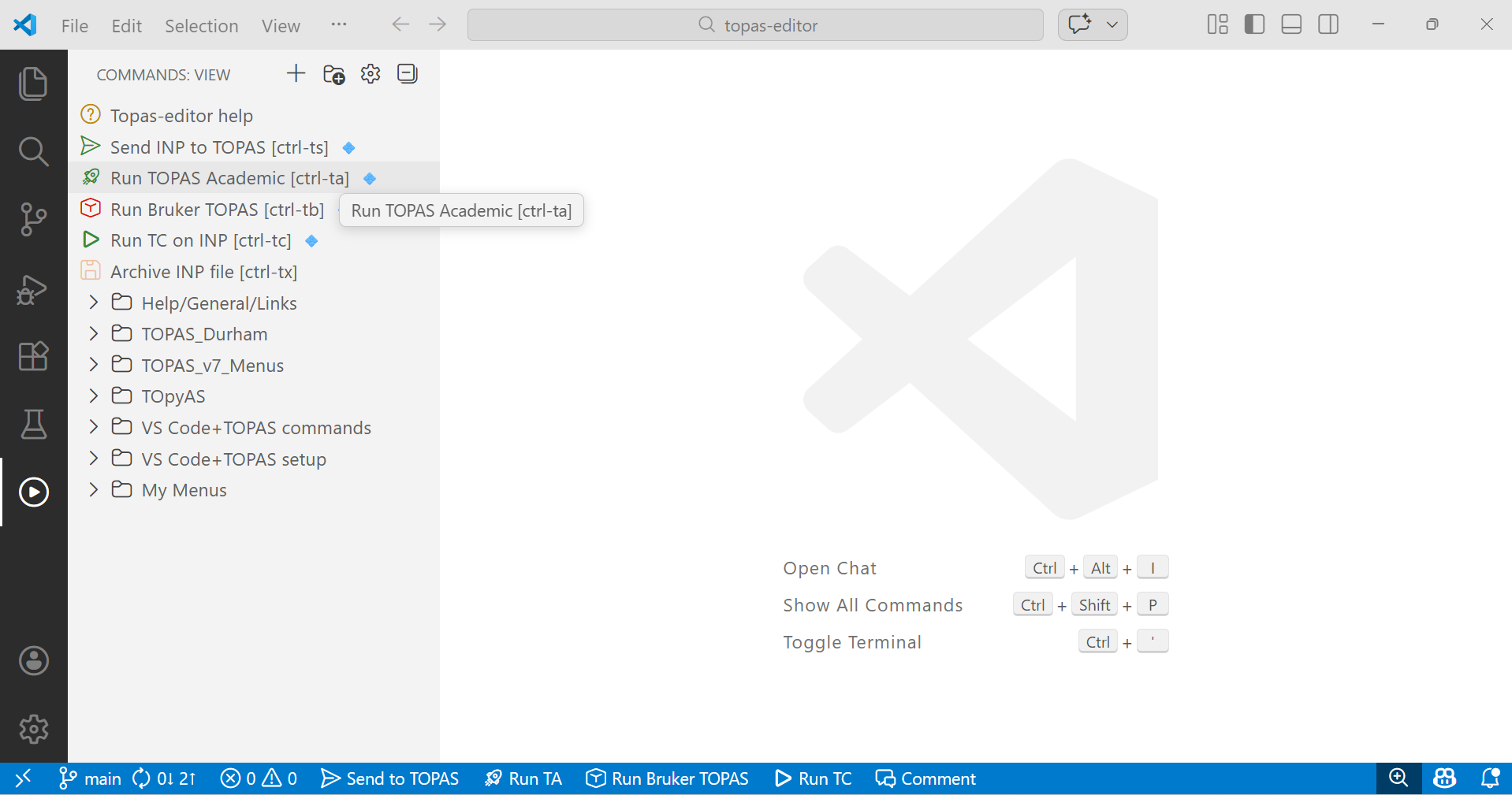
3. Launch TOPAS Academic or Bruker Topas by clicking on the green “Run TOPAS Academic” or red “Run Bruker TOPAS” as highlighted in the figure above. You can also launch these TOPAS versions with ctrl-ta or ctrl-tb (hold down ctrl key then type t then a), respectively. These commands are also available by clicking in the blue status bar at the bottom of the screen.

4. TOPAS will launch and will look something like the screenshot at point 14, but you won’t see the plot or zoom windows yet.

5. Switch back to the topas-editor window to prepare the INP file. The quickest way to do this is using the keyboard alt-tab shortcut.

6. We’ll now prepare an input (INP) file that contains all the instructions needed for a simple Rietveld Refinement.

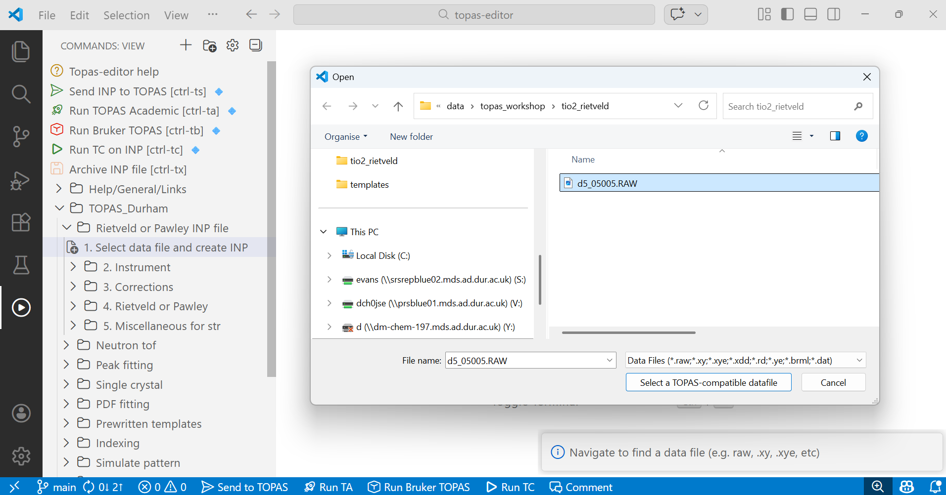
7. On the grey side menus click on the “TOPAS_Durham” tree item to expand it, then click on the “Rietveld or Pawley INP file” item. You’ll see a set of sub-menus labelled 1 to 5. You can create an INP file by clicking on each in term and making some choices. As you do this the corresponding instructions for Rietveld refinement will appear in the text window to the right.

First click on “Select data file and create INP”. A dialogue box will pop up. Navigate to select a TOPAS-compatible data file, here d5_005005.RAW. In the bottom right of the topas-editor screen you’ll see a pop-up information window. In general these windows contain instructions on what to do next, or a summary of the last thing you did. Click to select the file. Your screen should look like:

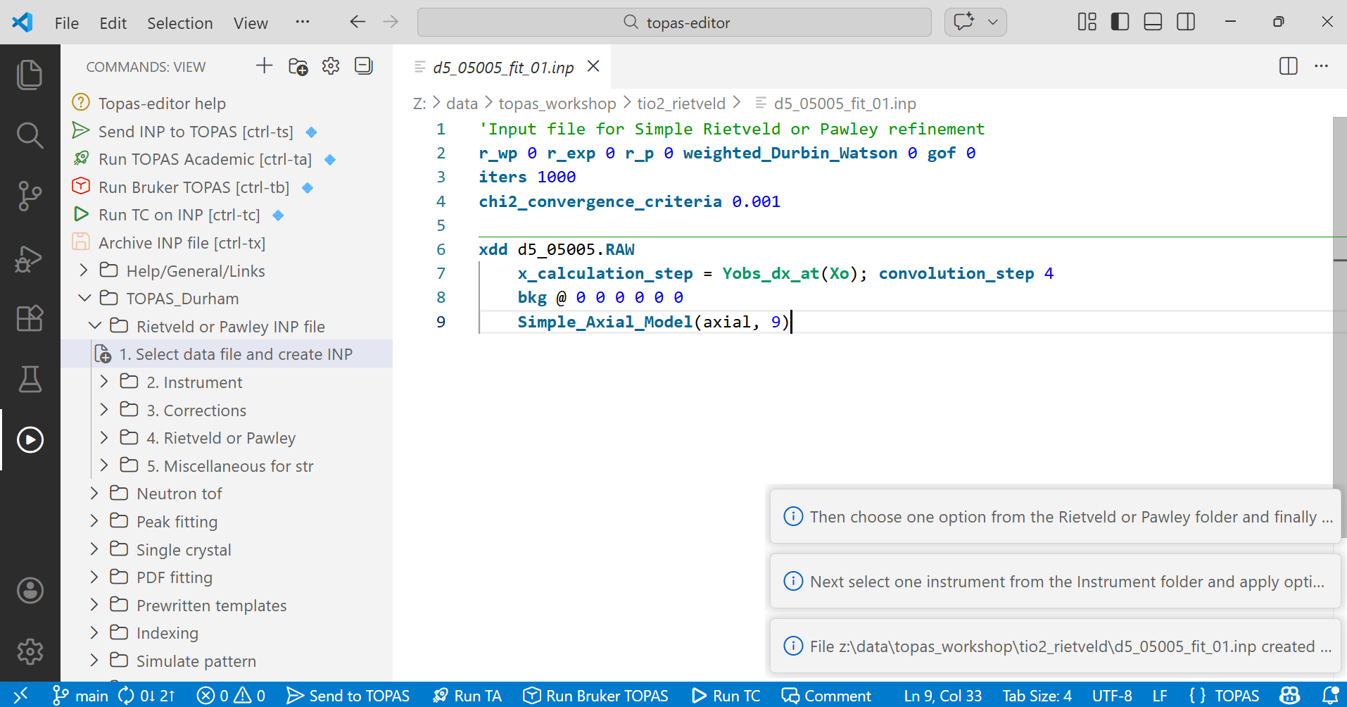
8. After selecting the data file your editor window will look something like the image below. It contains instructions about the refinement like the fit indicators, the number of iterations and the criterion for terminating the refinement at convergence. It then contains information about the data set, the points at which to compute the calculated pattern and a description for peak asymmetry. Note the instructions that appear temporarily in the bottom right. In the image they should be read from the bottom up. They tell you what to do next.

9. Next select the instrument by expanding tree item 2. Choose “BB_CuKa2_grapite_scint Durham d5000” – the diffractometer used to collect the data (traditional Bruker/Siemens d5000 diffractometer with Cu radiation, a graphite diffracted beam monochromator and a scintillation counter). The TOPAS description of this instrumetn will be inserted in the editor window. Note that you should only make one choice in this section. If you accidentally make multiple choices delete any inserted text in your INP file, then put the cursor at the end of the file.

10. Expand “3. Corrections” and click the “Refine sample height” option. Note that you could make multiple choices in this section, but parameters like zero point and sample height are highly correlated and should rarely be refined together. For a well-aligned modern instrument it’s normally sample height that dominates peak shifts in a Bragg-Brentano dataset.

Up until this point the process for a Rietveld and Pawley refinement is identical.

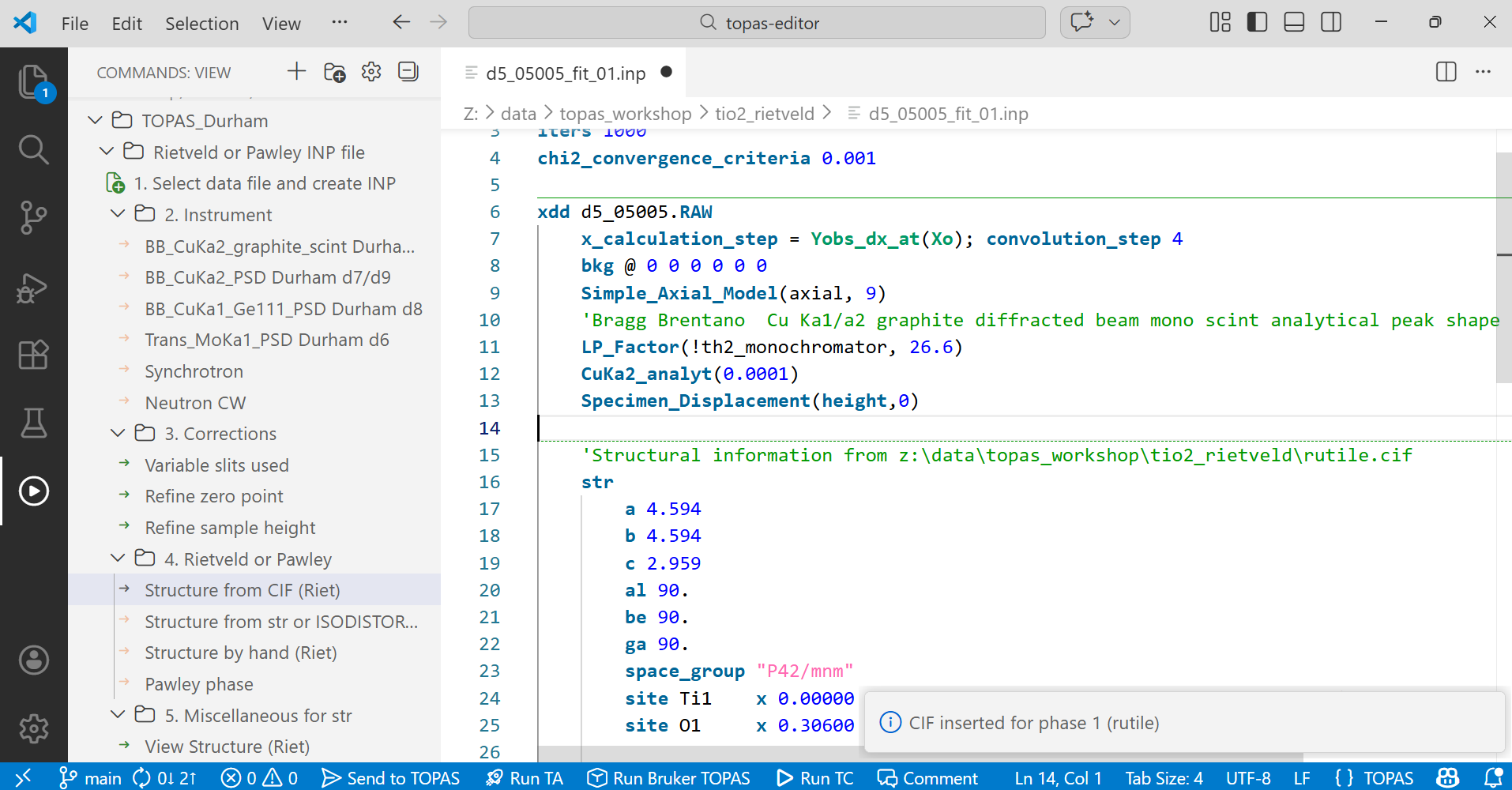
11. Expand “4. Rietveld or Pawley” and make one of four choices. For a Rietveld refinement you need a structural model. This can be inserted either from a CIF file, from an ISODISTORT str file, or you can create the structure step-by-step yourself. We have a CIF file rutile.cif so click on the first option, navigate to find the CIF, and open the file to insert it. This CIF reading method works for most structures. For molecular structures you could try Fabio’s CIF reader which is in the “Miscellaneous useful commands” tree and does some molecular clean-up operations.

At this point your file will look something like the image below, and contains all the information needed to start a simple Rietveld refinement, with a sensible initial set of parameters set to refine.

12. Take a minute to look through the file and the various instructions it contains. By default TOPAS keywords and most macros are colour coded in dark blue. Comment lines are flagged by starting the line with ‘ or by enclosing a block of text in /*….*/ and are coloured green; they’re really useful for storing notes about your work. Numbers are given in bright blue.

topas-editor has a number of other tricks to make visualising INP files easier. For example it puts a horizontal green line above each xdd section in the file, which contains the information about each individual data set being analysed. It puts a dashed green line before each str section, which contains information for each phase.

You can get a bit of information about many of the TOPAS keyword by hovering over dark blue text with your mouse. There’s more information in the technical reference. The technical reference is a wonderful information source, and is essential reading.

You can change things like the colour scheme used from items in the “VS Code + TOPAS commands” folder. You can access any of the TOPAS-specific VS Code commands by typing shift-ctrl-P and typing “topas” in the box that appears, select any of the commands to execute them. The most-used commands can be accessed by a right-click in the text window.

13. We now need to save this INP file and tell TOPAS we want to run a refinement based on the instructions it contains. Click on “Send to TOPAS” which is at the top of the side menus. Alternatively the same command is in the blue status bar at the bottom of the screen. Or you can type “ctrl-ts”. This command does two things: 1. a .backup file is created in case the refinement messes up; 2. The filename is written to a file called “launch_file.txt” in the main TOPAS directory; TOPAS constantly monitors this file so it knows what INP file you want to run.

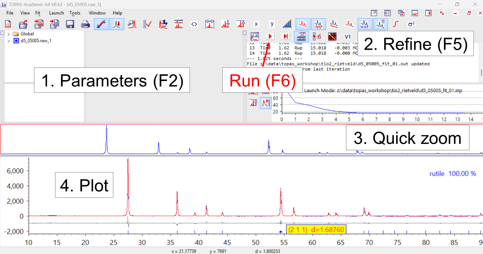
14. Switch to the TOPAS window (alt-tab as many times as needed). Your screen should look something like the image below, but without the powder pattern showing. The TOPAS gui has four different windows that are useful for this tutorial: 1. the Parameters window contains some information about the refinement; 2. the Refine window that is used for running the refinement and viewing the R-factor; 3. the Quick zoom and 4. Plot windows let you view the fit. At this stage you won’t see windows 3 & 4. If you don’t see windows 1 and 2, they can be toggled on and off with F2 and F5 keys, or you can display them from the “View” menu. If you drag windows to the edge of the main TOPAS window they will dock. I like the layout below.

In the Refine window you should see the name of the INP file written. If you’re using the Bruker version of TOPAS you may need to click on a “Rocket” icon in the Refine window to switch from gui mode to launch mode.

In the Refine window click on the red Run arrow to run the refinement (or hit F6). The data will be read in and the refinement performed. The Rwp will be plotted in the graph in the Refine window. In this case it converges to Rwp ~15 % in 12 least squares iterations (seconds on a typical PC). A dialogue box will appear asking if you want to update the original INP file with the results of the refinement (saved in a .out file). You can click “Yes”. If this later turns out to be a bad choice you can revert to the autosaved .backup file.

15. In the plot window you can zoom to look at different parts of the fit. You can hover over a tick mark to read the hkl indices. You can look on a linear, Sqrt, or log y-scale. Sqrt will emphasise weaker aspects of the data, and you should see random fluctuations in the difference plot at the end of the refinement on a Sqrt scale. The icons in the top bar let you control various aspects of the graphics, show the cumulative chi², show the background, etc.

16. Switch back to topas-editor (alt-tab). The INP file will have been automatically reloaded to include the results from this fit. Parameters that were set to refine will now have their numerical values coloured red so you can see them more clearly. For example, the background parameters which follow the keyword bkg will be red, as will parameters describing peak asymmetry (axial) and speciment displacement (height). TOPAS knew to refine these parameters as they contained parameter names in the INP you created. If a parameter is named but should be fixed in the refinement the name is preceeded by a !. For example, the monochromator angle, !th2_monochromator, is fixed at 26.6 degrees.

17. We could try refining the unit-cell parameters and an isotropic temperature factor on each site. We can do this by giving the relevant parameters names, or by using the @ symbol which tells TOPAS to create a parameter name automatically. Since TiO₂ is tetragonal we must keep the a and b cell parameters equated by giving them the same name (lpa below). Edit your file so it looks like the screen shot below. Note that topas-editor supports multiple cursors and column editing which is a super-quick way of making many changes in the file similtaneously. For example, if you hold down shift-alt and click after each word “beq” you get a series of cursors. If you type ” @” the @ symbol will be entered on each line. This makes editing INP files very quick. Hit esc to remove the multiple cursors when you’re done.

Sometimes columns in an INP file become misaligned so column editing is hard. There’s a topas-editor trick to sort this out: highlight the lines, right click, select “Align-columns” then choose the option to align by separator. Type space in the dialogue box then ok.

18. Save the INP file. As TOPAS already knows the name of the INP file you’re using you could do a regular save (ctrl-s) rather than “Send INP to TOPAS” (ctrl-ts). If you do this you won’t get a .backup file created.

19. Switch back to TOPAS (alt-tab), run the refinement again (you should get Rwp ~ 13.75 %), accept the results and switch back to topas-editor. You will see that the cell parameters and atomic displacement parameters are now coloured red indicating they have been refined.

20. There’s one free fractional coordinate in this structure – the x parameter of O; y is related by symmetry. Try refining this parameter by changing the oxygen line to read as follows:

site O1 x xo1 0.30600 y xo1 0.30600 z 0.00000 occ O 1.00000 beq @  0.12`

Here both x and y coordinates are given the same parameter name (xo1) which forces them to be identical. Alternatively you could change the O line to read as below. Here the y coordinate is set by a simple TOPAS equation. The “:0” after the equation is optional – it gets TOPAS to write the outcome of the equation in the INP file for you to check. You should get a Rwp of ~ 13.7 %. RBragg will be around 3.7 % and the goodness of fit, Sqrt(Chi²), around 1.3.

site O1 x xo1 0.30600 y =Get(x);:0.0 z 0.00000 occ O 1.00000 beq @ 0.12`

21. You might like to test the influence of different peak shapes, different numbers of background terms, refining a sample height correction instead of a zero point, etc. Try changing the parameter axial to values of 0 then 20 and fixing it (change parameter name to !axial) to see the influence of axial divergence on peak shape and refined unit-cell parameters.

22. Are you in a the global minimum? Try adding the lines below to the top section of the file to randomise the structure according to esd’s on parameters. TCHZ peak shape parameters are highly correlated, so this may diverge. Click the “stop” button when you’ve seen enough.

randomize_on_errors continue_after_convergence

23. At this point we’ve finished a default refinement. If you want to look at the errors on refined parameters add the key word “do_errors” at the top of the file and repeat the refinment. Errors will be appended to each refined parameter in the INP file as, for example, 4.593287`_0.000063. The second number is the standard uncertainty derived from the least squares fit, not a hard +/- range. The correlation matrix will also be written to the INP file. You can also view the correlation matrix in the GUI by clicking on the matrix icon in the refine window (next to v1). Beware correlations > 90%.

If you decide you don’t want to see the errors in the INP file you can remove them with ctrl-te.

The stability of least squares refinements in TOPAS comes in part from parameter limits that are used in the underlying maths. If parameters hit these limits then the esd’s reported no longer have any meaning. You will be warned about this by a LIMIT_MAX/MIN warning in the INP file. The model should be adjusted to remove these.

24. If you add the keyword “view_structure” in the str section of the INP file TOPAS will open a structure display window.

25. If you want to know more about the various commands in the INP file, you can get some information in a “hover help” window if you hover the cursor over dark blue text. There’s more information in the technical reference manual, which is linked from the Help side menu.

26. Other tutorials contain more information on what the various parts of the model are doing.

27. It’s not required, but it’s good practice to use indentation tabs in INP files according to “scope” to make them more readable. The process above does this by default. Overall instructions, generally at the top of the INP file, are not tabbed in. All the information that belongs to a given data set (xdd) is tabbed in by one unit (it has xdd scope). An xdd could contain multiple sructures (str) or other fitting commands; the information for each str has an extra tab. If your tabs mess up, you can highlight a block of text and type “tab” or “shift-tab” to move it right or left.

28. In some cases you might not need to use the gui version of TOPAS to visualise the refinement. If so, you can just type “ctrl-tc” in topas-editor. This will run the command line version of TOPAS on whatever INP file you have open, then reload from the .out file at the end of refinement.

29. If you have Matthew Rowles’ powder cif routines installed (see the TOPAS wiki), try saving a CIF file and viewing it in pdCIFplotter.

30. Optional extra work: hopefully everything went smoothly in this tutorial. When you analyse your own data you’re more likely to make mistakes in setting up the INP file or choosing what to refine. You could try deliberately making the following “mistakes” to learn how to trouble shoot.

a. Try typing the word “hello” somewhere in the INP file. It won’t be colour colded in topas-editor which is a hint it won’t be recognised by TOPAS. Run the refinement. Look at the error that appears in the Refine window. Open the log file and the error will also appear there. The line number TOPAS suggest for the error may be closer to the line number in the log file than the INP file. Sometimes TOPAS can only formally identify an error several lines after the line that caused the error.

b. Try refinining the x-coordinate on Ti. What happens to the calculated density? Why? Try putting the text “num_posns 0” after the site labels Ti1 and O1 and see what that tells you.

c. Try changing the space_group name to something non-sensical. What warning do you get in the INP file from topas-editor? What error does TOPAS give you?

d. It’s only really relevant for trigonal and hexagonal space groups, but try changing the x coordinate of O1 to 0.3333. What warning does topas-editor give you? If you run the refinement in TOPAS what error message do you now get?

e. Try moving the peak shape TCHZ_Peak_Type() line to the top of the INP file. Here it’s “scope” is incorrect – i.e. it’s not in a logical part of the INP file. What (cryptic) error message do you get?

f. Try changing the line that describes the emission profile to “CuKa1(0.0001)”. Look at the calculated peaks at high 2-theta.

g. It makes no crystallographic sense, but see what happens to the values and esd’s if you try refining the cell angles alpha, beta and gamma.

Pawley refinement from scratch

1. Performing a structure-free Pawley fit is very similar to a Rietveld refinement. Follow steps 1 to 10 above. If you have already done the Rietveld tutorial. you will be asked if you want to overwrite the existing INP file or create a new file. Choose to save your file as d5_05005_pawley_01.inp.

2. Alternatively you can save your existing Rietveld INP file as a new name and delete everything from the str line down, then place the cursor at the end of the file and proceed.

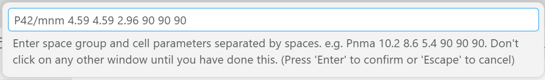
3. When you get to step 11 (tree item 4), click on “Pawley phase” instead of one of the “Structure…” choices. A dialogue box like the one below will appear at the top of the screen. Enter the space group and cell parameters as: “P42/mnm 4.59 4.59 2.96 90 90 90”. Be careful not to leave the VS Code window until you have entered these values. If do navigate away, click the menu item again, but then remove any duplicate lines from your INP file.

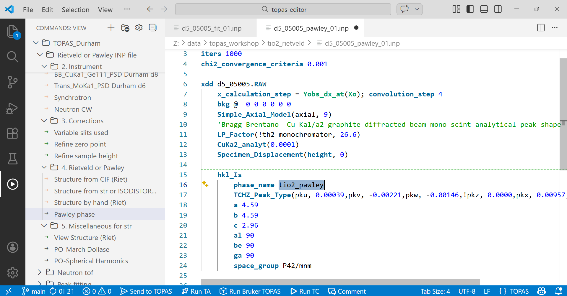
4. Your INP file should look something like the image below. If you like, change the phase_name to something sensible as in the highlighted text below.

5. Click “Send INP to TOPAS” (ctrl-ts). If TOPAS is not already open then click “Launch TOPAS Academic” (ctrl-ta). Switch to TOPAS (alt-tab), check that the correct INP filename is displayed in the Refine window, then press the red Run arrow. You should get Rwp ~ 22.8 %.

6. Set the cell parameters to refine (see section 17 above). Save and switch to TOPAS. You should then get Rwp = 14.7 % or lower. Try refining all the peak shape parameters except pkz (which correlates infinitely with other peak shape parameters). You should get Rwp ~ 13.1 %. Refined peak intensities will be listed in the INP file, immediately after the space_group line.

7. In addition to being a good check of space group and unit-cell parameters, Pawley fits give you an indication of the best agreement factors you might be able to achieve with a Rietveld fit for a given data set. Compare the Rwp and GoF to the equivalent Rietveld refinement above.

Rietveld or Pawley refinements from a template

Rather than creating an INP file from scratch, it’s often quickest to start from an earlier file or to work from a prewritten template. There are many templates distributed with topas-editor.

1. Download the data file and CIF file at the top of the page to your directory if you haven’t done the tutorials above.

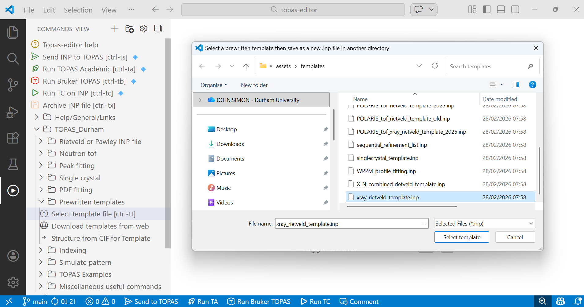
2. Navigate to the “TOPAS_Durham/Prewritten templates” folder in the left menus and click on “Select template file”. This will show you the templates available in topas-editor. If no files appear you can download templates from the “Download templates from web” menu. Select the “xray_rietveld_template.inp” file. Your screen will look something like the image below. After you click “Select template” a second dialogue box will appear asking you where you want to save the INP file. Navigate to the folder containing the data file and save with a suitable filename (e.g. d5_05005_template.inp).

3. Work your way through the INP file and replace any text highlighted in “-> purple after an arrow” with appropriate information for the TiO₂ example as given above. To save typing in structural information you can use the “Structure from CIF for Template” tree item to import the structural information. Make sure your cursor is at the point suggested in the INP file when you do this.

4. Click on “Send INP to TOPAS”, then run the refinement in TOPAS. Then follow the instructions in the Rietveld tutorial above.

5. There are templates set up for many of the most common types of analysis.

Cheat files

Typical INP files are: d5_05005_fit_01.inp and d5_05005_pawley_01.inp