TiO2 Index

Indexing

Files needed: d5_05005.raw (optionally your results from the peak fitting tutorial)

Learning outcomes: How to index a powder pattern in TOPAS from an INP file, then how to visualise the indexing results in the gui. See Alan’s J. Appl. Cryst. paper for details of the algorithms used.

TOPAS advantages: relatively robust to impurity peaks and (in my experience) TOPAS has never failed to index data that other routines have been able to index

1. In the topas-editor Durham TOPAS menus select Indexing, click to open an indexing template INP file and select the template from those presented. Save the file as tio2_index.inp.

2. Paste 2-theta and peak intensity values from the TiO₂ peak fitting tutorial into the section of the file labelled (i.e. below where it says “-> Paste here” in purple). If you haven’t done the peak fitting tutorial, then either use the values below or read the data file into TOPAS and use the “View/Search Peaks” routine.

	27.4908886	 1482.62496
	36.1397990	 601.766413
	39.2475489	 86.8457649
	41.2986185	 294.981236
	44.0960637	 113.069378
	54.3778813	 854.169193
	56.6781592	 263.059163
	62.8179927	 115.655192
	64.0972935	 126.977269
	65.5733631	 11.1309122
	69.0537887	 312.783969
	69.8586090	 143.643397
	72.4702535	 16.8939491
	76.5940077	 32.5261153
	79.8820917	 17.2423583
	82.3809157	 68.7857566
	84.2939417	 48.6984405
	87.5158448	 17.9090163
	89.5986433	 115.225801

3. Have a look through the INP file. It contains various options to control indexing, but most are commented out as they’re not needed in default cases. There are then a series of lines which tell TOPAS which of the 7 crystal systems to try.

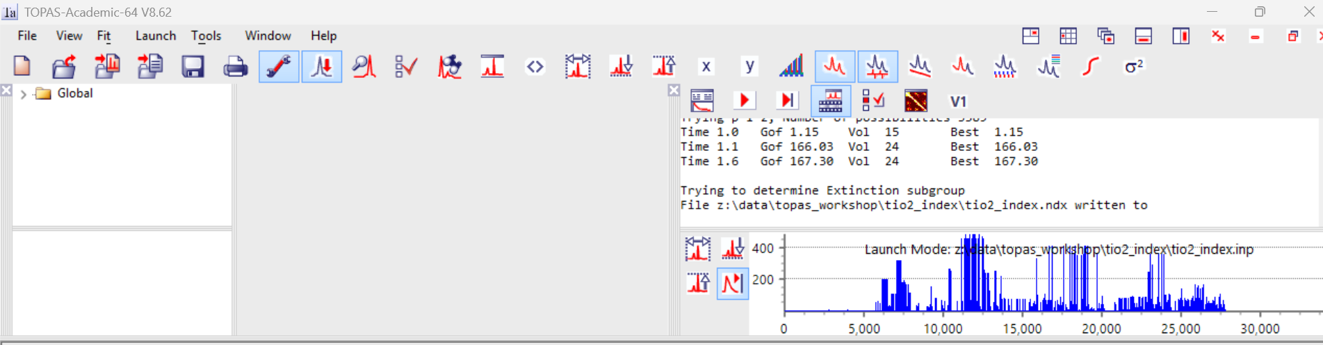
4. Click the “Send INP to TOPAS” icon (or ctrl-ts). Launch TOPAS (ctrl-ta) if it’s not already open and run the file (F6). On my computer it took 1.6 seconds for 28,000 indexing attempts. The screen should look like the image below where the blue plot shows the GoF for the different attempts. A good indication of correct indexing is when you see some cells with a high GoF that is significantly above the “noise” of bad cells – i.e. “spikes” in the plot below.

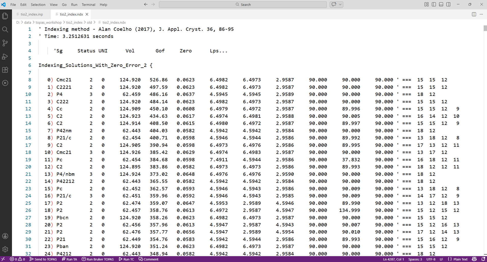
4. Indexing results get written to a file called tio2_index.ndx. Open this in topas-editor. It should look something like the image below. The unit-cells are ordered by their GoF. Here the best cells have a GoF ~ 500, and the worst around 0.14.

The columns in the file are explained in the technical reference. In brief: status can be 1, 2, 3 or 4 (1. weighting applied; 2. zero error attempt applied; 3. zero error attempt successful and impurity lines removal succesful; 4. impurity line(s) removed). The column “uni” gives the number of unindexed reflections. The final colums after ‘ === give an indication of the number of different h/k/l indices used in indexing. For cubic there will be one value, the number of non zero h²+k²+l² values used; for tetragonal there will be two entries (h²+k² and l²); for monoclinic there will be four (h², k², l², hk), etc. A value of -999 means the corresponding lattice parameter isn’t represented (e.g. if you have a 3 Angstrom cell parameter and the shortest d-spacing used is 4 Angstroms). At the end of the file there are tables of observed and predicted positions for the various reflections.

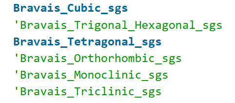
5. In this cae TOPAS has found a huge number of possible cells with very high GoF (>100). For this example it’s clear that best cells are all pseudo-tetragonal. For example the top solution has a and b essentially equal despite it being an orthorhombic space group. Their values are Sqrt(2) larger than those of solution 6. Try running the input file again with all but cubic and tetragonal systems excluded. i.e. the top of the INP file should look like:

6. The first cell listed should now be the one below, with a figure of merit around 400. TOPAS suggests a space group of P42nm. This has the same extinction conditions as P42/mnm, the true space group of TiO₂. The technical reference contains a table of space groups with the same conditions (search for “Extinction subgroups”). If you are going on to try structure solution as in other tutorials, it’s common to start with the highest symmetry space group and work your way down.

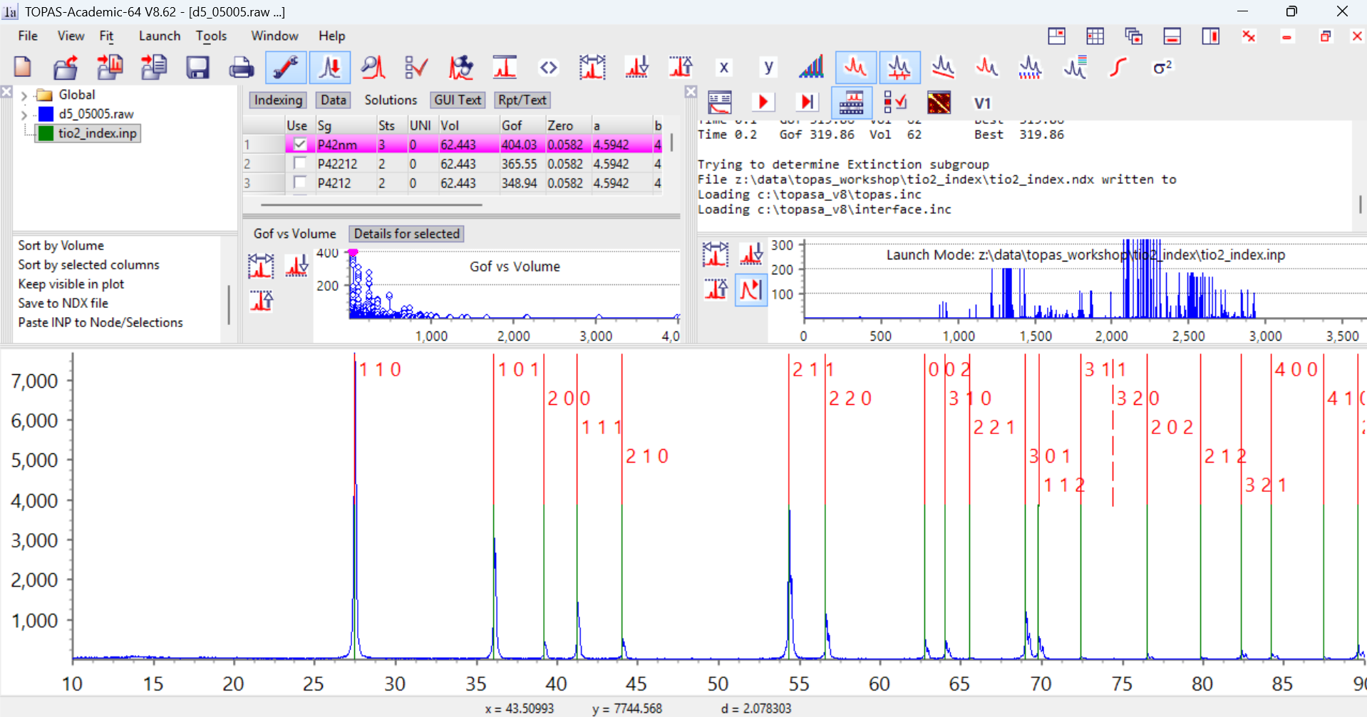
P42nm a=4.5946 c=2.9587

7. The TOPAS gui has a great feature for visualising the various unit cells and examining which peaks are indexed and which unindexed. Open tio2_index.ndx in topas-editor do ctrl-A to select all text, then ctrl-C to copy. Switch to TOPAS and type “ctrl-N” to delete any previously opened files. Go to “File/Load scan file” and read in the data from d5_05005.raw. Go to “File/Load INP file” and read in your tio2_index.inp file. The screen should look something like the image below. The green lines show the peak positions used in indexing.

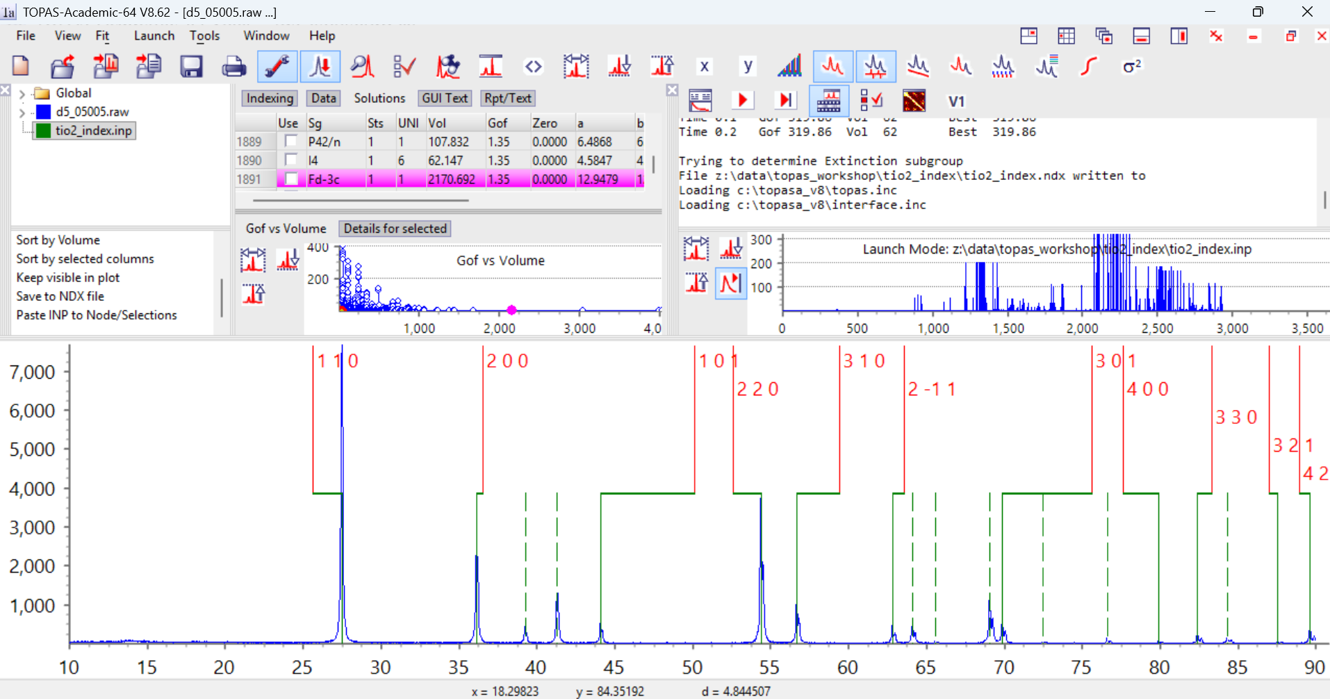
8. Now click on the green icon for the indexing range in the Parameters window (highlighted blue above). Click on the “Solutions” tab to the right. In the box in the bottom left of the Parameters window scroll to the bottom and you’ll see a command “Paste INP to Node/Selections”. Click on this and the results of the indexing are loaded into the gui from the clipboard. Your screen should now look like the image below.

On the right of the screen you can see the GoF values from the original indexing run. There are a series of high GoF solutions found around attempt number 2100 onwards. The graph in the Parameters window shows a plot of GoF vs cell volume from the ndx file. You’ll see some high GoF solutions with small cell volumes. If you click on the blue points in this graph you can visualise each unit-cell. Here I’ve clicked on the first cell (the pink dot). TOPAS displays the hkl values for each reflection as a red line above the green experimentally-determined position. In this case you’ll see that every green observed position has a red predicted reflection. There is only one predicted reflection (320) where there was no experimental peak. This is normally a good indication that the cell is correct.

9. If we look at the last cell in the list (GoF 0.14, terrible) there are 8 experimental reflections that aren’t indexed, marked by dashed green lines:

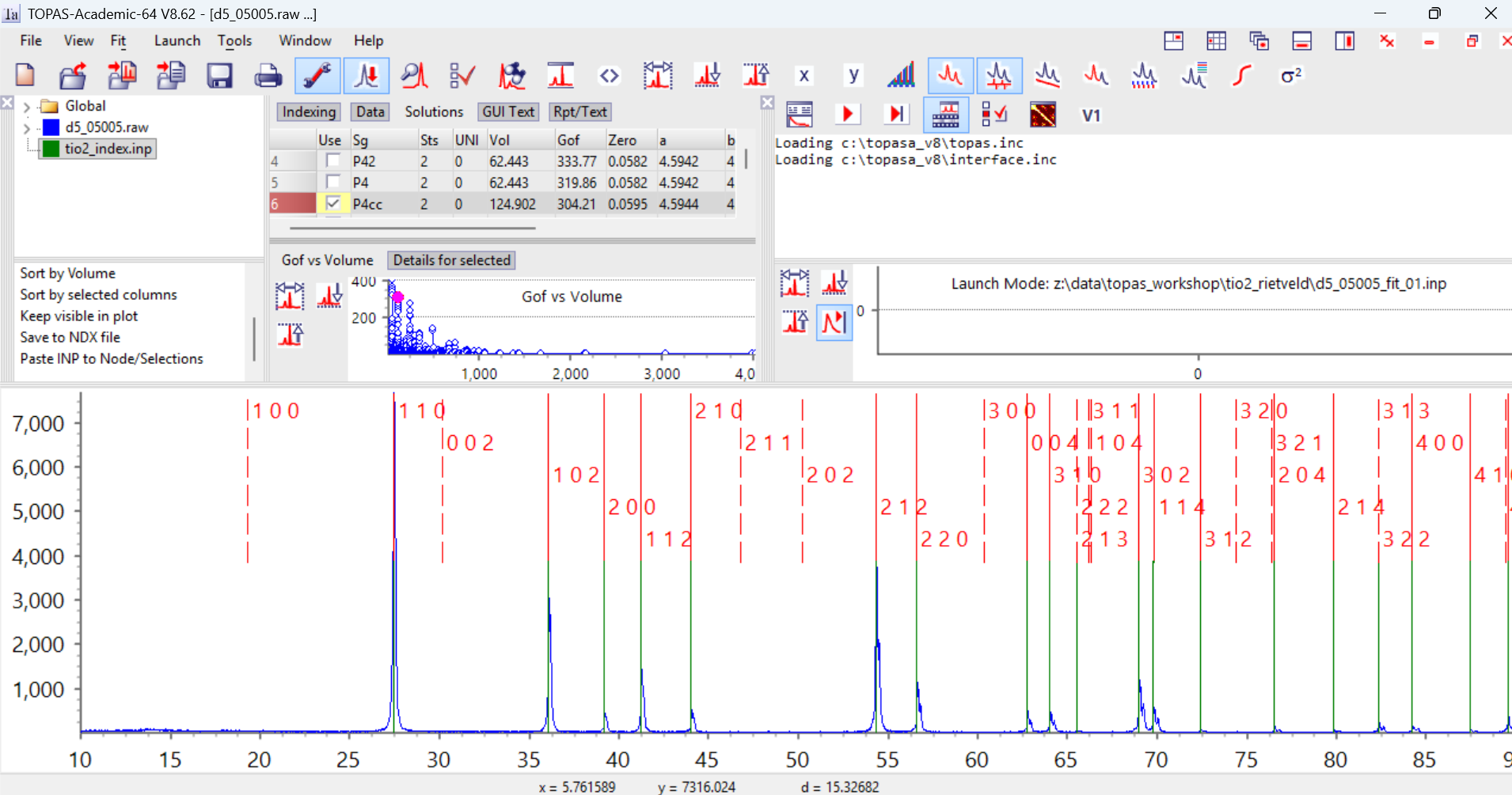
10. If we look at cell 6 in the list I got (your list might be slightly different to mine if you used slightly different 2-theta values), you’ll see it indexes all the reflections, but predicts a significant number of reflections that aren’t observed experimentally (the dashed red lines). It has a lower gof of ~304. This is actually a supercell of the true cell with the c-axis doubled, and you can see that reflections with l = odd aren’t unambiguously observed. A large number of predicted peaks where none are observed experimentally is often a sign of a unit cell that is sufficiently large that many of the peaks are indexed “accidentally” due to the density of reflections.

11. Beware. TOPAS gives a huge number of unit-cell suggestions. Many of them are equivalent cells. You could use a package such as delred to investigate this. For complex patterns lots of cells may “almost” fit the peak positions. Only one of them would allow you to solve/refine the structure correctly. Indexing is one of the hardest stages of structure solution. In my experience if the peak positions aren’t “perfect” at the indexing stage, structure solution is rarely succesful. Don’t waste time on a bad cell!

12. Extra work: Try a Pawley fit to the data using this cell and space group (i nstructions here). There are ways of using e.g. Python scripts to test each of the predicted cells in the .ndx file automatically.

13. Extra work: if you’re interested in indexing then try the same sort of protocol on any of the other data sets in the other tutorials.

14. Note also that the loading of tio2_index.inp into TA at step 7 is not possible when keywords that are not understood by the GUI are used. You can either simplify the INP file by commenting out commands, or create an indexing range manually using the option “Create Indexing Range” found by clicking on the “Global” treeview item of TA. Once the indexing range is created then the 2Th/Intensity peak values can be copied and pasted into the “Data” tab of TA. A window for displaying the indexing peak positions can be created using the TA menu option “Window/New Scan Window”. Thus graphical display of indexing solutions is always possible.