TOPAS Simple Least Squares
Topas Simple Least Squares
Files needed: data.xy; data_fit_01.inp; gaussian.xy; gaussian_fit_01.inp; gaussian_fit_02.inp
Learning Outcomes: Topas Academic is a program designed originally for powder diffraction data. However the flexible input file format mean that it can be used for a wide range of different types of data analysis. Here we’ll use it to fit the simple linear/quadratic/gaussian functions we explored in excel..
1. The file data_fit_01.inp contains the instructions needed to fit a straight line function. Save it to your working directory then open it in topas-editor. Save data.xy in the same directory. In topas-editor the INP file will look something like the screen shot below.
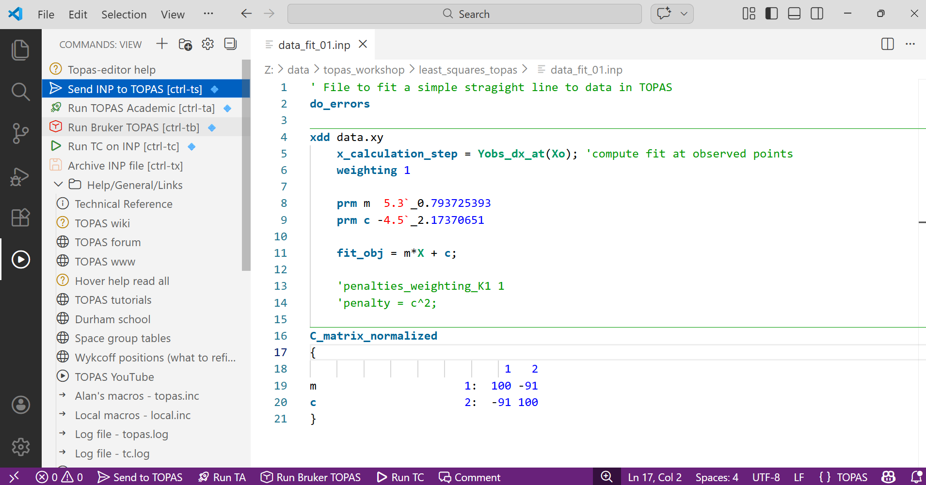
2. Read through the file. The format is relatively simple. The gradient and intercept of our y=mx+c function are defined as two parameters using the keyword “prm“. The name of the data files is specified using “xdd data.xy” (it’s a simple text file, open it and look). The line “weighting 1″ says to weight each data point equally. The line “fit_obj” contains the equation of the function we want to fit. The line “do_errors” tells TOPAS to calculate errors at the end of the refinement. Start m and c at any values you like by typing over the current values.
3. Click on the “Send INP to TOPAS” button in the left hand menu (highlighted blue above), or use ctrl-ts. This saves the file and tells TOPAS the filename containing the instructions for refinement.
4. Click on the appropriate “Run TOPAS” icon (e.g. highlighted greay above), or ctrl-ta or ctrl-tb. This launches TOPAS.
5. In TOPAS click on the red “Run” arrow in the refine window (F5 if you don’t see it). With Bruker TOPAS you may need to click a “rocket” icon in the refine window to set launch mode (i.e. read from INP file mode). The least squares refinement should run more or less instantly. Look at the observed and calculated lines in the graphical window. By default experimental points aren’t drawn but this can be changed by clicking on the filename in the Parameters window (F2 if you don’t see it), then on the “display” tab.
6. Go back to topas-editor. The results of the refinement should have loaded. You’ll see updated values for m and c in red text. After the “_” you’ll see the errors. At the bottom of the file you’ll see the correlation matrix. Compare the values to the ones you got in excel and to the correlation matrix we determined by hand in the lecture.
7. You could try a constrained refinement forcing the line going through the origin by fixing c to 0 with “prm !c 0″. You could force the gradient to be minus the intercept with the equation “prm c = -m;:0″, or by changing the fit_obj equation.
8. You could try a restrained refinment to guide the line through the origin by uncommenting the penalty lines. Now a penalty is applied proportional to c2. By changing the value of penalties_weighting_K1 to higher numbers you can “force” the line closer to the origin. This will be covered in lectures later in the week. Alternatively, you can edit the data file and add the point “0 0” at the top; this should give the same values as in the lecture.
9. The file “gaussian_01.inp” contains information to fit the simple Gaussian function that we used in excel. Run it using exactly the same protocol as above. We’ll later use similar protocols for fitting real diffraction data.
10. The file “gaussian_02.inp” contains exactly the same information using a “built in” gaussian peak shape function in TOPAS. Try changing positions and intensities as you did in excel to test the range of convergence. Try calculating errors.
11. Try changing the word “gauss_fwhm” to “lor_fwhm“. This forces TOPAS to fit a Lorentzian function (another function commonly used for fitting powder data) rather than a Gaussian. Note the difference in the shapes of the functions. We’ll return to this later in the week.