Size Strain

Size/Strain in topas

This page provides some information about performing size/strain analysis in topas and what the numbers mean.

1. If you want to do anything serious in this area you MUST read Balzar et al, J. Appl. Cryst. (2004), 37, 911-924.

2. Record a diffraction pattern of a highly crystalline sample (e.g. CeO2 that has been carefully annealed) under identical conditions to those that you want to use to record your diffraction data.

3. Analyse the CeO2 data in topas using e.g. a tchz peak type. The file linked here is for d9_00260 (Pawley fit of CeO2 data recorded to 140 degrees with v20 slits and 0.02 mm detector slit with the Sol-X). It gave a peak shape of:

Simple_Axial_Model(!axial, 9.02216`)
TCHZ_Peak_Type(!pku, 0.00039`,!pkv, -0.00221`,!pkw, -0.00146`,!pkz 0.00081`,!pkx, 0.00957`,!pky, 0.03386`)

The file linked here is for d8_02838 (Pawley fit of CeO2 data on d8, 5-140 degrees, 1 deg slits, vantec, step 0.0085059 degrees). It gave a peak shape of:

Simple_Axial_Model(!axial, 11.38115`)
TCHZ_Peak_Type(!pku,-0.00879`, !pkv, 0.00263`, !pkw, -0.00241`, !pkz, 0.00789`, !pkx, 0.02559`, !pky, 0.00597`)

4. Record your data under the same conditions as CeO2. To perform a full size/strain analysis you should use the peak shape determined in 3 and the macros below:

/*
LVol_FWHM_CS_G_L(k, lvol, kf, lvolf, csgc, csgv, cslc, cslv)
Calculates FWHM and IB (integral breadth) based volume-weighted column heights (LVol).
[k, lvol]: shape factor (fixed to 1), integral breadth based LVol.
[kf, lvolf]: shape factor (defaults to 0.89), FWHM based LVol.
[csgc, csgv]: Parameter name, Gaussian component.

Integral breadth based LVol is equivalent to DV as reported by Balzar or DR for Rietveld) (223 reported)

e0_from_Strain(e0, sgc, sgv, slc, slv)
Calculates e0 according to Balzar 1999
[sgc, sgv]: gaussian strain and value
[slc, slv]: lorentzian strain and value
*/

Simple_Axial_Model(!axial, 9.02216`)
TCHZ_Peak_Type(!pku, 0.00039`,!pkv, -0.00221`,!pkw, -0.00146`,!pkz, 0.00081`,!pkx, 0.00957`,!pky, 0.03386`)

LVol_FWHM_CS_G_L(1, 22.06386`, 0.89, 26.81884`, csgc, 50.47297`, cslc, 48.19244`)
e0_from_Strain( 0.00299`, sgc, 0.00016`, slc, 0.01196`)

5. An example file (ESRF data from the 2004 Round Robin publication) is linked here. Using this method of analysis in topas academic 2 gave DV of 224.9 for CeO2 against a published value of 223. Ignoring strain DV values were 221/219.

Interpreting Values

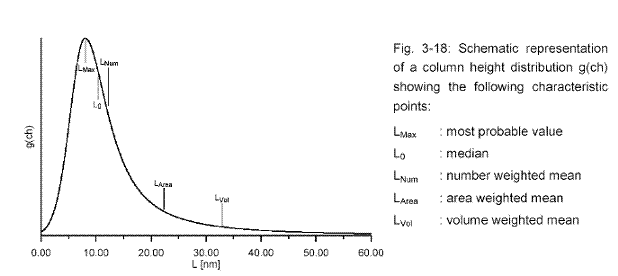
This is hard as different methods of analysis report different quantities. Diffraction measures volume weighted mean column heights (see the topas user manual). These differ from other quantities as shown in the figure below.

The LVol_FWHM_CS_G_L(k,DV,k,Dfwhm,gaus_size,val,lor_size,val) macro above gives the volume weighted mean column height as the second number (here 22.1 nm) based on integral breadth (the recommended method). This quantity is called LVOL by Alan and DV or DR in the Balzar paper. The second number (26.8) is based on fwhm and is not recommened. The last two numbers are the values you would get using just a CS_L(@,val) and CS_G(@,val) macros for Lorentzian/Gaussian size broadening. The conversion factors are detailed in the topas manual.

The second macro applies a Gaussian (0.00016) and Lorentzian (0.01196) strain broadening and reports the single value e (0.00299) as defined by Balzar (Voigt-function model in diffraction line-broadening analysis. – Microstructure Analysis from Diffraction, edited by R. L. Snyder, H. J. Bunge, and J. Fiala, International Union ofCrystallography, 1999) and also Balzar (2004).

It’s hard to relate DV to the average radius of particles because one is approximating a distribution of particle sizes (e.g. a Lognormal distribution as above) by a single quantity. Balzar states that the average radius (R) is related to DV by the expression:

DV=1.5*R(1+c)^3

Thus for a monodisperse spherical system DV=228 gives R=152 A; for a more typical lognormal distribution with c=0.2 one would get R=87.96 A. The error comes in replacing the histogram in the figure above by a single value.

The corresponding equation for DA (area weighted) for comparison with other methods of analysis is:

DA=(4/3)*R(1+c)^2

N.B. for very broad distributions of particles (high values of c) one can get superlorentzian peaks (i.e. tails fall off very slowly).