Tutorial Nano Size
Size Strain – FePt Nanoparticles
Files needed: d9_00233.raw, d9_00607.raw
Learning outcomes: This tutorial shows how information on the size of nanoparticles can be obtained. Make sure you have completed the CeoO2 tutorial before attempting this one. The double Voigt method used has significant limitations. It strictly doesn’t apply when the sample has a dispersion of particle sizes (e.g. a lognormal distribution) and ignores broadening due to defects or strain. These issues are discussed in the more in-depth WPPM tutorial.
1. Save the files above in your working directory.
2. Go through the menu for a Simple Pawley refinement.
3. Select one of the data files above.
4. The data were recorded on the Durham d9. Select this diffractometer.
5. For d9_00233 the spacegroup is Fm3m with a~3.85 Angstroms; for d9_00607 you can use a tetragonal cell in P4/mmm with a~3.85, c~3.75 Angstroms.
6. The instrumental peak shape for this measurement was determined using CeO2 and is:
Simple_Axial_Model(!axial, 9.02216`)
TCHZ_Peak_Type(!pku, 0.00039`,!pkv, -0.00221`,!pkw, -0.00146`,!pkz, 0.00081`,!pkx, 0.00957`,!pky, 0.03386`)
7 Use “Save/send to topas” button and refine in topas. The calculated peak shape should be far sharper than the experimental.
8. Introduce the following macro to describe sample broadening due to size. The various terms are defined here.
LVol_FWHM_CS_G_L(1, 4489.51014, 0.89, 5424.90744, csgc, 10000, cslc, 10000)9. Refine again. You should get a much lower wRp and LVolof 1.79 nm; for monodispersed spheres diameter=4*l/3=2.39 nm. Analysis of 257 particles by TEM gave an average size of 2.36 nm with sigma of 0.15 for this sample (around 7 nm for d9_00607.raw). Particles in d9_00607.raw are partially crystallographically ordered (hence the extra peaks) and contain significant stacking faults.
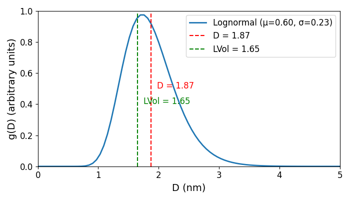
10. You might like to try the WPPM approach with this sample if you have the macros available. Add the lines below to your INP files. You should get mu = 0.60, sigma = 0.23 which corresponds to the lognormal distribution below. Removing the assumption of equally sized particles changes the size estimate slightly (LVol changes to 1.65(5) nm).
prm mu  0.601887167`_0.0241782649 min 0.5 max = Min(2 Val + .02, 5); val_on_continue = Rand(1, 3);
prm si  0.22942163`_0.014273086 min .01 max = Min(2 Val + .01, 1); val_on_continue = Rand(.1, 1);
prm !Diameter = Exp(mu+si^2/2); :  1.87424194`_0.045725604
prm !StanDev = (Exp(2*mu+si^2)*(Exp(si^2)-1))^(1/2); :  0.435712103`_0.031092778
prm !LSur = (2/3)*Exp(mu+2.5*si^2); :  1.38819972`_0.0405311758
prm !LVol = (3/4)*Exp(mu+3.5*si^2); :  1.64612668`_0.0548514079
prm !Lambda = Exp(mu+3.5*si^2); :  2.19483557`_0.0731352106
WPPM_Sphere_LogNormDIST(, mu, , si)