Tutorial fundamental params

Fundamental parameters peak shape fitting

Learning outcomes: This tutorial explores the use of fundamental parameters to describe peak shapes. You will compare the results of using an empirical pseudo voigt function to using direct convolutions that describe contributions from the instrument and sample.

There is some more information on fundamental parameters in the Y₂O₃ Rietveld tutorial.

Files needed: ceo2.xdd, ceo2_01.cif

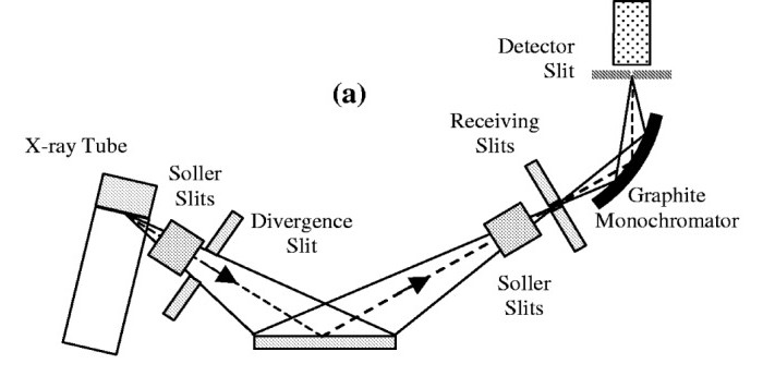
Information: powder diffraction data were collected on CeO₂ using a traditional diffractometer with a Cu tube as depicted below (taken from Cheary, Coelho and Cline, 2004). For the tutorial we will assume a monochromator angle of 26.6 degrees. For axial contributions to the peak shape we will assume 1 degree divergence slits, a 0.1 mm detector slit, a filament length of 12 mm, a sample length of 20 mm, 5 degree primary and secondary Soller slits.

Topas advantages: complex peak shapes can be simulated using a small number of physically sensible parameters.

1. Save the datafile in your working directory. Do a standard Rietveld fit using a TCHZ peak shape function. You can use BB_CuKa2_graphite_scint as the instrument type. Refine zero point, cell parameter and isotropic temperature factors. A 17 parameter fit with 6 peak shape parameters should give Rwp ~8.5%.

2. Edit your file so you can fit the data using a fundamental parameters approach: (a) change the emission profile to CuKa5(0.0001). (b) comment out the TCHZ peak shape lines. (c) comment out the Simple_Axial_Model() line. (d) Add the lines below to describe the instrument in the xdd section. Hoverhelp in topas-editor will tell you what these parameters mean.

	Radius(173)
	Full_Axial_Model(12, 20, 12, 5.1, 5.1)
	Divergence(1)
	Slit_Width(0.1)

3. You should get Rwp ~44%. Look at the fit. You’ll see that the calculated peaks, which are based solely on the calculated instrumental contribution, are too sharp.

4. Introduce the lines below to the str section. They describe Lorentzian and Gaussian sample broadening contributions due to crystallite size and strain. You should get an Rwp around 9.43%.

		CS_L(@, 100)
		Strain_L(@, 0.0001)
		CS_G(@, 100)
		Strain_G(@, 0.0001)

5. Try refining the secondary Soller angle from its initial value of 5.1 degrees (put an @ symbol in front of the number). You should get Rwp ~6.7%.

6. Look at the Gaussian contributions to the peak shape compared to the Lorentzian in the INP file. You should see that the Gaussian size is a large number (low broadening) and the strain is small (also low broadening) compared to the Lorentzian contributions. Try commenting out these lines. You should find that the Rwp is essentially unchanged, suggesting these parameters aren’t needed.

7. This is a 14 parameter fit, with 3 parameters describing the peak shape. The fit is better than the 7 parameter empirical model.

Extra work

8. We chose to just refine the secondary Soller angle here as it is sufficient to give a good peak shape description. You could try changing the values of other instrumental descriptors to see how they influence peak shape. In practice several of the parameters are highly correlated and it’s sensible to fix some of them to expected values. Other parameters have little effect on the peak shape over a wide range of values, so should also be fixed.

9. You should be able to get an equivalent fit using the LVOL_FWHM_CS_G_L() and e0_from_Strain() macros that will be in your INP file if you set it up using topas-editor.

10. The file here is one way of doing the tutorial.