Magnetic GA structure solution

Magnetic Structure Determination using a Genetic Algorithm

Learning Outcome: This tutorial uses a Genetic Algorithm to determine the magnetic structure and magnetic symmetry of (Ce_0.78La_0.22)₂O₂MnSe₂ [Ainsworth, C. M.; Wang, C.-H.; Johnston, H. E.; McCabe, E. E.; Tucker, M. G.; Brand, H. E.; Evans, J. S. O. Inorganic chemistry 2015, 54, 7230.]. The essential idea is that the GA lets you determine which of the magnetic modes in a P1 description are actually needed to fit the observed magnetic peaks. From the modes needed it is then possible to determine the true magnetic symmetry of the material and develop a simpler structural description.

Prerequsites: We strongly recommend you try one of the simple tutorials on fitting time-of-flight neutron data before attempting this tutorial.

Pre-tutorial preparation

This tutorial requires python 2.7 and some additional packages for data analysis. The easiest way to install these is via the Enthought Canopy python 2.7 distribution available at https://store.enthought.com/downloads/#default, though other Python distributions can also be used. The xlsxwriter package (for writing to Microsoft Excel files) is also required and can be installed by typing “pip install xlsxwriter” into the Canopy command prompt (open Canopy and go to: Tools -> Canopy Command Prompt). Ensure that the Keep Directory Synced to Editor option is checked in the drop down menu in the top right of your python command window.

Extract all the files from the .zip linked above to a directory on your computer.

If you haven’t updated your jEdit recently you might need to set colour coding on .inp0 files so you can view them like normal .inp files. Go to you user/.jedit/modes directory and edit the file called catalog. Append “.inp0” to the list on the “MODE NAME” line.

If you’re missing macros to allow files to run try going to the macros page on the topas wiki.

Tutorial

Data were collected on (Ce_0.78La_0.22)₂O₂MnSe₂ at 30 K using the GEM time-of-flight neutron diffractometer at ISIS. GEM collects data in 6 banks over a range of d-spacings. Bank 6 has the highest resolution and smallest d-spacing range. Bank 3 contains data over a larger d-spacing range at reasonably high resolution and contains a number of strong magnetic reflections

Determine the magnetic unit cell. In a general case the first step in magnetic structure determination is do determine a cell which fits both the nuclear and magnetic peaks. In this case the magnetic cell is identical to the nuclear cell. You can confirm this by performing a Pawley fit of e.g. one bank with clear magnetic peaks and one high resolution bank where cell parameters are well determined. Use file find_mag_p1_Pawley.inp to check all the 12 K peaks are predicted by the nuclear cell. Later in the tutorial you’ll see that the nuclear cell doesn’t predict intensity for several of the peaks..
Use ISODISTORT to obtain a description of the magnetic structure in magnetic spacegroup 1.1. Go to http://stokes.byu.edu/iso/isodistort.php and:
1. Load find_mag_cmca_01.cif as the parent phase and click OK.
2. Under Types of distortion to be considered check Mn and Ce magnetic modes and uncheck strain modes. Then click “Change”.
3. Under Method 3 select SG P1 and click OK (leave basis = {(1,0,0),(0,1,0),(0,0,1)})
4. On the distorted structure page check “1.1 P1, basis={(0,0,1),(0,1,0),(-1,0,0)}, origin=(0,0,0), s=2, i=32” and click OK.
5. On the distortion page check “TOPAS.str” and click OK to save the file. Rename it find_mag_cmca_01-mag_1pt1.str.
The next step is to set up a template “inp0” file for the magnetic GA to fit the bank 3 GEM data. To save you time there is a pre-prepared file find_mn_p1_01_ga_all_modes.inp0. The format of this file should be familiar if you’ve done some of the time-of-flight tutorials. Open the file and look through the various sections. The file is set up so you can include other data banks and includes structural descriptions of a minor Ce2O2Se impurity and V from the sample can. The important section to look at is labelled “strs that go into every data set”. The first structure described is that of (Ce0.78La0.22)2O2MnSe2 using symmetry modes. The information here is basically copy and pasted from find_mag_cmca_01-mag_1pt1.str. The edits that have been made are:
1. In the “mode definitions” section the “magrand” command has been added to allow magnetic modes to anneal.
2. In the “mode-dependent sites” section site labels have been changed to Ce+3 and Mn+2.
3. Each atom has been give an isotropic temperature factor of 0.25.
4. To exclude displacive modes in the GA the “’#GAexclude” tag has been added after each displacive mode. Displacive mode parameters start with an ‘a’ while magnetic mode parameters start with ‘mm’.
5. You can check if there are errors in the .inp0 by saving a copy as temp.inp and running it through topas. Magnetic mode amplitudes are zero in this file so it represents a nuclear-only fit. You should get Rwp ~15.2% and see that 8 peaks at 6.6ms, 7.1ms, 7.3ms, 10.0ms, 11.7ms, 13.5ms, 15.3ms and 15.8ms have zero calculated intensity with the nuclear model..
Magnetic phase transitions typically involve distortion modes belonging to a single irrep. Therefore we will conduct a GA where the irreps (rather than the individual modes) are the attributes. In order to do this we need to tell the GA program which modes belong to which irrep. The script get_irrep_block_lists.py contains a module that will detect this automatically. Paste the magnetic mode information from find_mn_p1_01_ga_all_modes.inp0 into get_irrep_block_lists.py. Be careful not to overwrite the dummy line at the bottom of the mode text. In this case this has already been done for you.
The script gacontrol_mn.py controls the magnetic GA. For this simple example we only need to edit lines 21-26 of the script:
1. On line 21 set the number of repeat experiments. Currently this is set to 1. Increase the 2nd number if you want more repeats (and expect to wait longer for your results!). It is often useful to confirm that the same result is obtained in repeat runs in order to be sure your GA has found the model with the lowest fitness possible.
2. On line 23 enter the name of the folder you want results output to. Repeat experiments are automatically suffixed _1, _2 etc.
3. On line 24 enter the directory you are working in (where these files are) on your computer.
4. On line 25 check that the directory matches the directory of your tc.exe TOPAS application.
5. On line 26 set the penalty or penalties you wish to apply per irrep active you wish to apply. In this case you will find any number between 7 and 0.1 will isolate a single irrep. In a real example you may have to trial a few different penalties to establish the right level to isolate a single irrep.
6. In a real example you would change the name of the inp0 file on line 84.
7. Advanced Notes (these can be skipped):
  1. Lines 28-32 contain additional GA controls, each with a comment. If you find the facts window that appears while the GA runs annoying, you can turn it off here for example. Try a GA with mode attributes if you wish (you will notice that the best modes come mostly but not entirely from the same irrep and that the importance of each mode is best considered alongside other important modes and not in isolation).
  2. Lines 45-54 contain GA parameters concerning the probability of mutation and crossover events occurring, the size of the population and the length of time the algorithm will last. There is a comment next to each explaining its purpose. Change them if you wish (you might be able to improve the speed of the GA with good choices). The block crossover parameters are not relevant for an irrep based GA and you will receive a warning if you try to set blockcxbitcxratio to a value other than 0.
  3. Lines 57-58 define the total time of the GA. You can reduce these if you like although you will reduce the probability of finding the best solution. In this case the best irrep will probably be identified very early on and the GA will end 10 minutes after that.
  4. Lines 91-94 define the fitness function for this system under “if key==”find””. The fitness function is defined as (Rwp/fitmin)+(penalty_per_irrep*irrep_count). Normalising the Rwp helps in setting an appropriate penalty per irrep. If you don’t wish to do this change the value of fitmin to 1 and rescale your penalty per irrep as appropriate. Try different fitness functions if you like.
Run the GA by pressing the green run button at the top of the Canopy editor window. You should be in the correct directory if you synced your directory to your editor but if not use cd <tutorial directory> in your python command prompt. On a slow computer you might need to be a little patient as there is lots of computation going on in the background. You can expect to wait around 30s per generation on an ordinary desktop PC. If canopy crashes you can select “Run/Restart kernel” from the menus. Sometimes the information in the python editor window disappears off the bottom of the screen. Scroll down if you want to see it.
As the GA runs look in the facts window and the plot window. These may be minimised by default. In the plot window the green line shows the fitness of the best member of each population, the red the worst and the blue the average. In generation 0 all members have no modes turned on an the fitness is ~9.5. This should reduce as the GA runs. The facts box is colour coded so it goes green when an improvement is made in the population, red when the population stagnates and amber in between. The window tells you how many generations it has been since the fit improved. In generation 0 you shoud see “Best fitness” is 15.2. This corresponds to the Rwp value we obtained above for the nuclear only fit. After about 5-10 generations you should see bestfitness ~ 2 and Best Rwp ~1.7%. This is the correct solution.
The python window at the bottom of your Canopy environment will alert you with “GA stopped” when the run has finished. On average you can expect the best irrep will be isolated in about 100s. This means the GA will end after 700s. Monitor the “facts” window that appears if you wish to see your current best modepool, its Rwp and fitness amongst other things. You may wish to use the ‘Stop at end of Generation’ button if you do not wish to wait any longer.
You can see which modes are identified by looking in the facts window. However many times you repeat the experiment, you will almost certainly notice that the best modepool reads: “[40, 41, 42, 88, 89, 90, 117, 140, 141, 164, 165, 188, 189, 212, 213]” with Rwp = 1.695%. This is very close to the Rwp = 1.6% achieved when all 216 modes are allowed to be active. You should see that “Best fitness penalty” is 1 because a single mY2- irrep is active. You can confirm this by opening find_mn_p1_01_ga_all_modes.out and noticing that the active modes correspond to only mY2-. For more information, various files are written to your directory:
1. A .rep file that reports details of every candidate in every generation throughout the GA.
2. A .amp file that reports the mode amplitudes of every active mode in every evaluation made in the GA.
3. A .err file that reports the most recent evaluation made by tc.exe (use this in case of an error occurring in a TOPAS evaluation).
4. The last .inp file evaluated in the GA.
5. The last .out file from the final evaluation of the GA.
6. A .pic file that reports a few important facts about your GA: The best (lowest fitness) modepool obtained by the GA; The time that it appeared (in seconds); The number of modes in the best modepool; The number of irreps in the best modepool; The irreps active in the best modepool; The Rwp of the best modepool; The total number of evaluations made by the GA; The reason the GA stopped (this will almost certainly read 600.00000, meaning the GA stopped because no improvement had been made for 600 s).
At the end of the GA you can see how good the fit is to the data by running find_mn_p1_01_ga_mY2-_modes.inp through topas. This produces find_mn_p1_01_ga_mY2-_modes.cif although some formatting changes have been made so it can be read by FINDSYM. You should see an excellent fit to the experimental data.
Now we have identified that the magnetic distortion modes needed to fit the experimental data we can find the real magnetic SG symmetry. The file find_mn_p1_01_ga_mY2-_modes.cif is our best magnetic SG 1.1 model (using only mY2- modes). We use FINDSYM to find the real magnetic SG:
1. Go to http://stokes.byu.edu/iso/findsym.php.
2. Under “Import Data” load find_mn_p1_01_ga_mY2-_modes.cif and click Ok
3. On the FINDSYM page search with default tolerances by pressing OK at the bottom of the page
4. Scroll down the output. About halfway down you will notice FINDSYM has returned a model in magnetic SG 62.455
5. At the bottom of the output you will find a CIF file. Copy it and save it as find_mn_62pt455_mY2-_modes.cif if you wish.
(Optional) If you didn’t have the .cif file you could find the same information using ISODISTORT:
1. Go to http://stokes.byu.edu/iso/isodistort.php
2. Load find_mag_cmca_01.cif as the parent phase and click OK.
3. Under Types of distortion to be considered check Mn and Ce magnetic modes and uncheck strain modes. Then click “Change”.
4. Using Method 2 select the Y-point to superpose and click OK
5. On the irreducible representation page select “mY2-“ and click OK
6. On the distorted structure page accept only basis option: “P1 (a) 62.455 P_Cnma, basis={(0,1,0),(1,0,0),(0,0,-1)}, origin=(1/4,1/4,0), s=2, i=2, k-active= (1,0,0)” and click OK.
7. On the distortion page check CIF file and OK to save file (as find_mn_62pt455_mY2-_modes.cif) if you wish.
Now that we have found the true magnetic space group we can do a final Rietveld refinement and confirm that the R-factor is as good as a more complex description in 1.1. The file CHW055_MAG_jsoe_my2m_01.inp is set up to do this. All the data banks have now been included in the refinement. Under “mode definitions” the 15 mY2- modes we identified earlier are listed, however only two modes are freely refining. The other modes are either dependent on those two modes or fixed to zero amplitude. You will notice the fit to the data is still very good.
1. Try refining all 15 parameters freely. To do this delete the “!” before any fixed modes and set all the current values to 0. You should notice the Rwp is not significantly better than with just two parameters. Look at the mode amplitudes – it should be clear that there is only one non-zero mode amplitude needed for the Fe modes. The relationship between Ce mode amplitudes is harder to spot by eye.
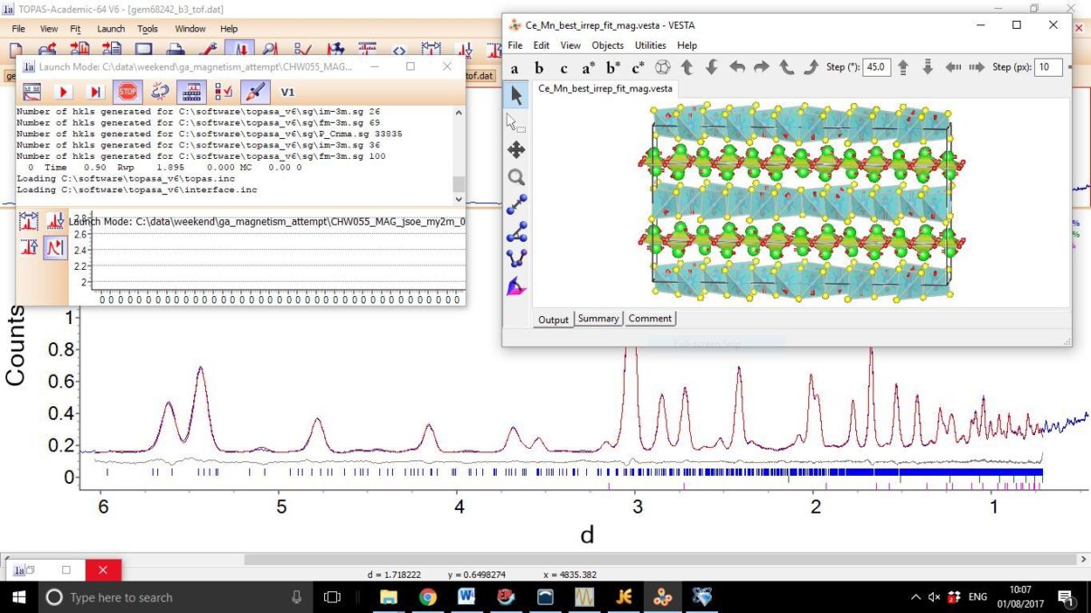
2. Lastly look at the view distortion tool in TOPAS (or load Ce_Mn_best_irrep_fit_mag.vesta in to VESTA if you have it). You should notice the AFM alignment of Fe moments along each layer. The Ce moments are arranged in pairs with opposite moments when adjacent to corner sharing MnSe4 tetrahedra. Ce moments point directly along the layer when adjacent to edge sharing MnSe4 tetrahedra.
3. A screenshot of what you should see is appended below.
In a real example you will not know which penalty per irrep values will return the single best irrep. It may be that you are not even be sure the distortion is controlled by a single irrep. To investigate this:
1. Enter a list of penalty per irreps to try on line 24 of gacontrol_mn.py: “[10, 7, 1, 0.1, 0.01, 0]”.
2. Try each penalty per irrep 5 times by entering on line 21: “num_runs = 5”.
3. Run the GA again (answer “y” to remove existing files). This will run for around 24 hours.
4. You can analyse the results using the template Excel file provided: GA_results_sum.xlsx. You will also notice paste_me.xlsx has now appeared in your working directory. Paste each section of text into the space provided in the “results” sheet in GA_results_sum.xlsx (each group appears in order of penalty per irrep as defined earlier).
Key outputs from your GA runs will be in the summary sheet. Open terms such as “Average modesum” indicate the average achieved across all 5 repeat runs at that penalty. Bracketed terms such as “(Average modesum)” exclude any GA runs that do not match the lowest fitness model found. For lower values of penalty per irrep you are more likely to find inconsistent results for a GA over a fixed timeframe. You will notice that in the plot of (average irrepsum) vs (average Rwp) that the Rwp falls sharply on the introduction of the 1st mY2- irrep but hardly falls at all for subsequent irreps. Also inspect the three graphs that plot penalty per irrep. You will notice that penalties in the range 7-0.1 all produce a final irrep count of one. This means that in order for a second irrep to be introduced into the model the penalty must be very low because it provides almost no improvement to the Rwp. Conversely the penalty must be very high to exclude the mY2- irrep because the there is a big improvement in Rwp. Only when the penalty term completely dominates the fitness function ((Rwp/1.6)+(penperirrep*irrepcount)) is the lowest fitness obtained for 0 irreps. The clear indication from this analysis is the magnetic distortion is controlled by the mY2- irrep alone.