TOF
OPAS-Academic Tutorial
TOF calibration / refinement of CeO2
CeO2 data are used in this example from ISIS HRPD and comprises a sharp pattern TA-Tutorials\data\tof\sh1.xy1 and a broad patterns TA-Tutorials\data\br1.xy1 which form part of the size-strain round robin conducted by the IUCr CPD 1 (Balzar, 2001). Section 3.2.2 of the TA Users Manual also discusses this data.
In this tutorial the sharp pattern will be fitted first in order to obtain instrument constants. These constants will then be used to fit to the broad pattern with the instrument constants fixed in order to determine specimen broadening.
Note that there are now better functions available for describing the instrumental peak shape of HRPD than the exponentials used here, but these probably don’t have signficant impact for the tutorial as the sample contribution from CeO2 dominates. See the Topas wiki (search “tof” and you should find a file “time_of_flight_tof_isis_instrument_standard_files”).
Fitting to the sharp data
A Pawley refinement will be performed on the sharp pattern as structural data is not sought; peak shapes are important here.
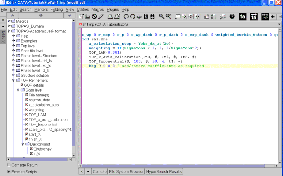
Open the jEdit XInsert treeview item “TOPAS-Academic, INP format/TOF Refinement”.
Work your way down the treeview clicking on the items x_calculation_step, weighting, TOF_LAM, TOF_x_axis_calibration, TOF_Exponential and a Chubychev background. Note, there’s no need to include neutron_data and the TOF scaling of D_spacing^4 as we are doing a Pawley refinement.
The jEdit screen should now look like:

Notice the # character in the TOF_x_axis_calibration macro. Typically the User finds these constants from the instrument local contacts and it would be a matter of entering the right ones. In this case however we are going to determine the constants starting from an approximate t1 of 1548018, thus change the line to look like the following:
TOF_x_axis_calibration(t0, 0, t1, 1548018, t2, 0)
Notice the removal of the characters ! and thus we will be refining on the three parameters t0, t1 and t2.
Open the XInsert node called “Phase level- hkl_Is”. Here we will insert the Pawley phase. Position the cursor on the bkg line and Click on hkl_Is, Cubic, and space_group. Clicking on space_group inserts the keyword space_group plus a $ siign. Change the dollar sign to the space group “Fm-3m”. Change the Cubic line to correspond the known CeO2 lattice parameter which wont be refined, it should look like:
Cubic(5.4103)
Go to the “TOF Refinement/Phase level” and click on TOF_PV; this represents part of the instrument function. Its a PseudoVoigt with a FWHM that varies in X-axis as a function of D_spacing. It may be useful at this stage to view the TOF_PV macro in the file TOPAS.INC. Load it into jEdit from the XInsert node of “TOPAS-Academic, INP format/Help/Standard macros – Topas.inc” and search for TOF_PV by pressing Alt-s or use the jEdit menu option “Search/Find”.
The jEdit screen should now look like:

Press Alt-b to go back to the sh1.inp file.
Now we will do a preliminary refinement on sh1.inp.
You will notice that the fit is poor with a background that looks wrong. Looking at the pattern we notice that some of the observed data at low and high tof space is oscillating considerably.
Go to the XInsert node of “TOF Refinement” and insert a start_X of 800000 and a finish_X of 5000000. This will remove the low and high parts of the pattern which is causing the poor background fit.
This brings up the important point that “Refinement” typically comprise a series of refinements each including small modifications to the INP flie leading to progressively better fits.
Alt-Tab to TA and refine again and save the parameter values by answering Yes to the prompt.
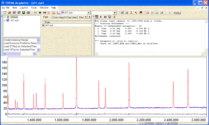
The fit should be good with an Rwp of 8.8%. Increase the number of background Chubychev coefficients to 6 by adding three zeros ‘0’ to the end of the bkg line and then refine again; the Rwp should refine to around 8.67%.
Zoom into a region of the scan and the fit should look something like:

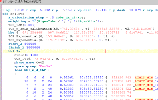
Alt-Tab back to jEdit and the INP file should look like:

This completes fitting to the sharp data and determining the instrument constants found in the TOF_x_axis_calibration line, the TOF_Exponential line and the TOF_PV line.
Fitting to the broad data
Even though it is fast to work down the treeview and insert required items; it is even more expeditious to use the sh1.inp file as a template and to modify it to accomodate a new data set.
Save the sh1.inp file as br1.inp and change the xdd line to include the data br1.xye.
Remove the refine unique ‘@’ characters from the TOF_Exponential lines and the TOF_PV line. Stop refining on the t0, t1 and t2 parameters by prepending the character ! to the parameters names in the TOF_x_axis_calibration line, ie.
TOF_x_axis_calibration(!t0,-403.55857, !t1, 1545934.99243, !t2,-218.54623)
Place an @ sign in the Cubic line to refine on the cubic lattice parameter, ie.
Cubic(@ 5.4103)
The fit is poor as seen below and clearly the peaks of br1.xye are much broader than the calculated pattern. We will now include some specimen broadening.

Place the curcor somewhere after the hkl_Is keyword and click on the XInsert items of TOF_CS_G and TOF_CS_L which are found under “TOF Refinement/Phase level”.
Save, Alt-Tab to TA and perform a refinement; you should notice a very good fit with an Rwp of 4.86%.
