Boehmite
TOPAS-Academic Tutorial
Variable Counting Time data – Rietveld
Variable counting time data of Boehmite was recorded at CSIRO Melbourne Australia by Ian Madsen. The calculated pattern Yc in terms of a calculated pattern collected at fixed counting time per step, Ycf, at data point i is given by:
Yc(i)=t(i) Ycf(i)
where t is the dwell time at data point i. TA loads the data (*.vct files) and modifies the observed pattern Yobs to match that of fixed counting time. To maintain the correct weighting and hence correct parameter errors the following is minimized:
(Yobs(i)/t(i) – Ycf(i))^2 (t(i)^2 / Yobs(i))
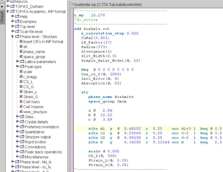
Open the XInsert mode “Topas-Academic, INP format” and work down the nodes inserting items such that the jEdit screen looks like the following:

Note that an x_calculation_step is necessary as the x-axis values are contained in the vct file. Looking into the vct file shows that the x-axis is at equal values and thus the data could be changed to equal step size using rebin_with_dx_of .025. Equal step size data is more computationally efficient to process and in a structure solution sense rebin_with_dx_of may increase computational speed.
The text “CuKa2(0.001)” was typed in; it corresponds to a macro which loads the emission profile file CuKa2.lam. It could have been loaded using the XInsert node node “Scan file level / Emission profile” but as one gets familiar with the data structures it is sometimes just as easy to simply use the keyboard for short text entries.
The structural parameters could have easily come from a CIF file but for such a small structure it is just as expeditious to use the XInsert node of “Sites” and type in the values.

The background is noisy at low 2Th angles as seen in the Ln plot; this is due to the shorter counting time at low angles.
Note that the parameter values started far from their refined values and that the refinement routine managed to bring them to converge in a few iterations . This is a characteristic of TOPAS-Academic that is most beneficial.
*.vct files are catered for in TA, however the refinement could have also been performed by first transforming the data to an *.xye file comprising three columns of x-axis values, Yobs values (which in this case would be equal to Yobs(i)/t(i)) and error values (which in this case would be (t(i)^2 / Yobs(i))).
